China vs. the US: Which GDP is bigger?

Has China yet surpassed the United States in aggregate economic power? Perhaps not.

Although China’s GDP, at market prices and exchange rates, is still much lower than that of the United States, the opposite is true if the calculation is made at the international purchasing power parity (PPP) prices (using the newly updated Penn World Tables). And China has been growing much faster.

If the objective is to compare national economic power (rather than standard of living), though, the PPP figure arguably overstates the power of low-income countries. A simple adjustment, relating to the Balassa-Samuelson (1964) effect, suggests that China may still be slightly behind the United States.

China’s population is much larger than that of the United States, but its average living standards are still well behind. Combining population and average output, GDP is often cited in standard or journalistic comparisons as a convenient summary measure of aggregate national economic power. Of course, power has many dimensions: political, military, technological, and so on. But even if one takes GDP as a single indicator, there are different ways of using it to make the comparison.

If the comparison is made at market prices and exchange rates, the United States is still well ahead of China.  By this metric, China’s GDP reached only 77 percent of US GDP in 2021 and has actually been falling since then (see blue line in figure below).

But few economists would recommend use of market prices and exchange rates for international comparisons of national accounts, instead preferring to use purchasing power parities (PPP). PPP calculations, which have long been carried out for the Penn World Table (PWT, Feenstra et al. 2015) on a multi-country basis, apply common international prices, matched for quality, to the various goods and services that make up GDP. They are invaluable not least because they help eliminate the distorting effect of transitory fluctuations in exchange rates (cf. Honohan 2020).

The new version (11.0) of the PWT, published recently, provides an updated and revised estimate of output in different countries valued at PPPs. These PPP calculations are the gold standard for making cross-country comparisons of average standards of living. China’s per capita GDP is less than 30 percent of that of the United States. But, with its much larger population, China’s total GDP has been ahead of that in the United States since 2016. This is shown by the red line in the figure above. By 2023 (the latest date in PWT 11.0) China’s GDP had reached more than 124 percent of that of the United States.

It is worth noting that, if we take national economic power to include a country’s capacity to match others across a range of products, and not just on the ones for which it happens to be relatively productive, PPP likely tends to exaggerate the attributes of low-income countries on this dimension. The Balassa-Samuelson (1964) effect of lower average price levels in low-income countries is a symptom of this tendency.

The leading hypothesis to explain the Balassa-Samuelson effect is that low-income countries are relatively less efficient in producing high-tech tradable manufacturing goods, with the result that less of these appear in the GDP of low-income countries and are relatively more expensive than low-tech goods and services (iPhones versus haircuts, for example).

Because the production pattern of a low-income country tends to reflect the sectors in which it is efficient, despite their relative price being lower, applying the (higher) international (PPP) relative price to these goods lifts the apparent GDP of a lower income country—and the more these prices are lifted, the less efficient that economy is.

If, instead, two countries were to produce goods and services in the same proportions, the ratio of the low-income country’s GDP to that of the high-income country would be much lower (see the appendix for diagrammatic illustration). Thus, the relative inefficiency of the low-income country would be more evident. Arguably, this would be a better measure of relative economic power.

Furthermore, a country’s ability to produce high-tech tradable manufacturing goods and services is more likely to be important in projecting economic power than its ability (given available production possibilities) to produce non-tradable goods and services. If attempted by government policy, such a projection would likely require a shift towards the production of tradable goods despite the high cost of doing so. Although the relatively low price of non-tradable items helps affordability and living standards, these low prices and the higher production of these items that results is a symptom of weakness.

These considerations suggest that, if one is to use GDP as an indicator of a country’s aggregate economic power, some discount is needed relative to the PPP calculations to avoid overstating the economic power of low-income countries. One simple procedure is to adjust the GDP at PPP of each country by subtracting the average Balassa-Samuelson effect estimated from a cross-country regression.[1]

That is how the orange line in the figure has been computed for China.[2] Note that, despite having removed the Balassa-Samuelson effect, the adjusted figure is still well above the blue line (GDP at market prices and exchange rates). However, it is substantially lower than the unadjusted PPP and suggests that China’s aggregate economic power may still have been only 91 percent of that of the United States in 2023.

Admittedly, if the Balassa-Samuelson effect partly results from factors other than productivity differentials, this might be too much of an adjustment.

And this might be especially true for China. After all, several important parts of the Chinese economy are technologically highly advanced. But large swaths of the Chinese economy are still relatively low tech, and the average price level in China is much lower than that in the United States. Although the simple two-sector model sketched here clearly doesn’t do justice to the complexity of China today, the applicability of the Balassa-Samuelson argument remains plausible.

To be sure, China continues to grow economically at a faster rate and is catching up in average standards to other large, advanced economies, and the size of the adjustment will decline as this happens. It may be merely a curiosity that, on this overall measure of economic power, it has not yet overtaken the United States.

Nevertheless, if one wants to use GDP as a crude indicator of a country’s economic power, it seems unwise to ignore these quantitatively important implications of the productivity explanation, whether for China or other countries.

Appendix

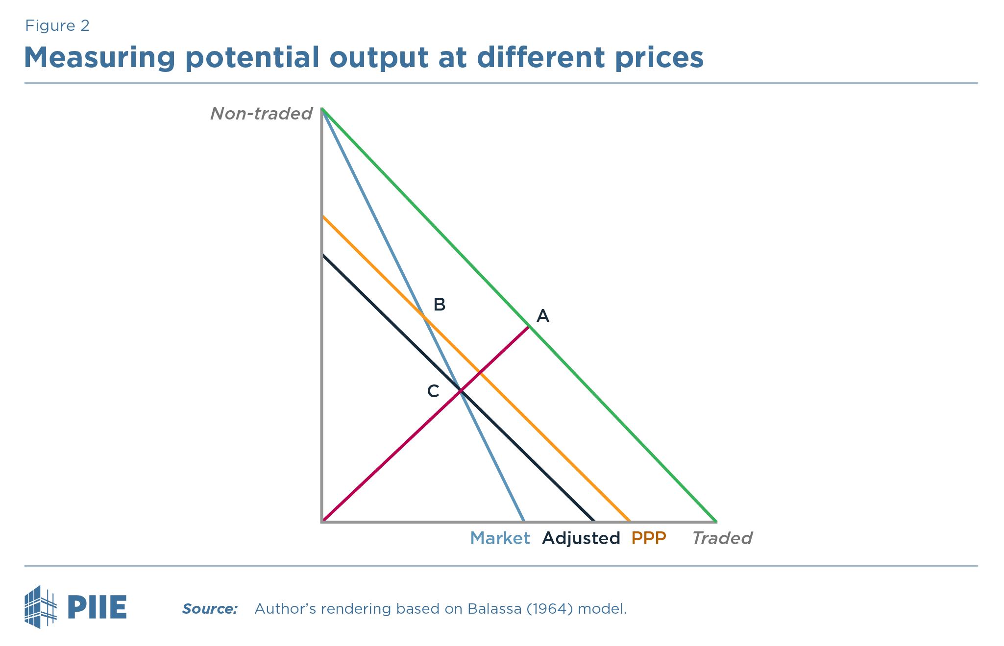
The reasoning is illustrated in the accompanying diagram showing the production possibilities for two countries, based on a simple model of the type employed six decades ago by Balassa (1964). Two goods are produced under conditions of constant unit costs (marginal rates of transformation). The rich country’s production possibility curve is the outermost line (in green); suppose A is the combination of tradable and nontradable goods produced in that country. The low productivity country’s production possibility curve is the blue line, on which we take B as the actual point chosen, with the output of tradable goods at B lower than at A. Then, if the poor country sought to produce the same ratio of tradable to nontradable goods, it would be at C. A PPP calculation for output (using any tradable-to-nontradable price lower than that prevailing in the low productivity country) gives a lower value to C than to B. For example, using the rich country’s prices, these can be read off the horizontal axis at the points marked “PPP” and “Adjusted.” This is a Paasche-type bias, but one that is arguably worse than usual since the bias increases mechanically with the cost inefficiency. That will not do if we are trying to gauge the overall economic potential or power of a country. In order to eliminate the bias, we should calculate at C, not B. The simple adjustment proposed in the text seeks to apply this logic to the much more complex world of multiple products and countries. Note that valuing actual output B at market prices (giving the point marked “Market”) would introduce the opposite (Laspeyres-type) bias.

Notes

1. The alternative of using market prices and exchange rates (on the argument that economic power in practice depends on international market prices) is unattractive. Not only would that reintroduce the problem that market exchange rates are volatile and often far from fundamental values (even if averaged over a few years), but it would entail a bias in the opposite direction to that which arises with PPP by ignoring the potential for the pattern of production to be shifted by government policy aiming at projection of economic power.

2. The figure is drawn assuming that the slope of the Balassa-Samuelson effect is 0.25, which is the point estimate of α in a regression of the form \(\ln(P_{it})=\alpha\ln(Y_{it})\) (plus a constant term), where P is the PPP price level, Y is the PWT output measure of GDP at PPP divided by population, for country i and year t. This is in line with previous literature (cf. Cheung et al. 2017).

References

Balassa, Bela. 1964. The Purchasing Power Parity Doctrine: A Reappraisal. Journal of Political Economy 72: 584–96.

Cheung, Yin-Wong, Menzie Chinn, and Xin Nong. 2017. Estimating Currency Misalignment using the Penn Effect: It Is Not As Simple As it Looks. International Finance 20: 222–42.

Feenstra, Robert C., Robert Inklaar, and Marcel P. Timmer. 2015. The Next Generation of the Penn World Table. American Economic Review, 105(10): 3150-82.

Honohan, Patrick. 2020. Using Purchasing Power Parities to Compare Countries: Strengths and Shortcomings. PIIE Policy Brief 20-16. (Washington, DC: Peterson Institute for International Economics). November.

Samuelson, Paul. 1964. Theoretical Notes on Trade Problems. Review of Economics and Statistics 46: 145–54.

Data sources

For GDP at PPP: Penn World Tables

For GDP at market prices: World Bank World Development Indicators

For population: Federal Reserve Bank at St. Louis data for China and the United States (accessed November 8, 2025).